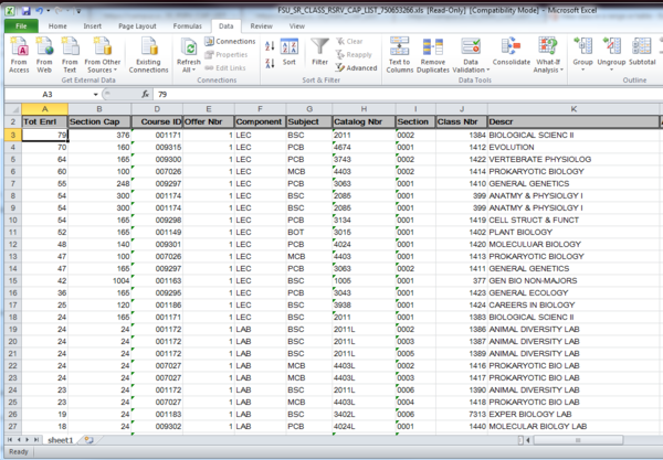
Queries allow you to generate reports based on whatever data elements you choose to include. The example below is an FSU_SR_CLASS query that uses reserve capacity data to generate report results. Further down the page, some examples of how to format results in Excel are shown.
Navigation
Log on to Student Central. Go to Main Menu>Reporting Tools>Query>Query Viewer
Steps
1. In the Search By field, type FSU_SR_CLASS.

2. Click Search. The Query Viewer/Search Results appear.
NOTE: The FSU_SR_CLASS category includes data elements that return reports related to scheduling data.
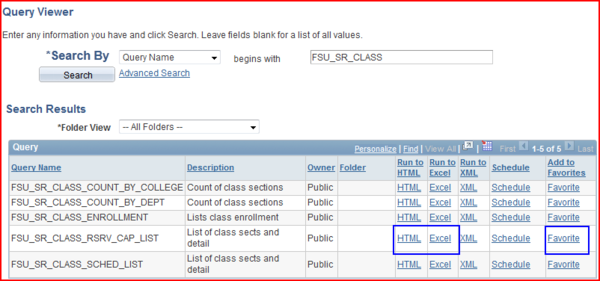
3. Choose a query to run: Run to HTML, Run to Excel, or Run to XML. Prompt fields appear in which to enter criteria.
NOTE: If you select Run to Excel, the resulting data is exported directly to Excel. If your computer blocks pop-ups, you may be prompted by the browser to approve the download. Approve this action for the download to complete. Do not select the Run to Excel option if Excel is not installed on your computer.
NOTE: You can add a query to your favorites list for quick navigation to the queries you run frequently.
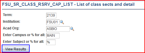
4. When you select Run to HTML or Run to Excel, an interface appears displaying fields for entering search criteria.
NOTE: Search-criteria field options vary depending on the specific query. The FSU_SR_CLASS_RSRV_CAP_LIST selection provides an example of the class reserve-capacity query's search criteria:
- Term-The term value is equivalent to the term value used in scheduling. Example: 2139 is Fall 2013.
- Institution-The institution value is always FSU01.
- Acad Org-The academic organization value limits the search to only those units you specify. Click the Look Up button (magnifying glass) to search for the necessary academic organization/s. Always provide a value here to limit your results.
- Enter campus or % for all-The % is a wildcard value in this system. Entering % returns courses for all campuses. To filter other campuses from the search, enter one of the three campuses (i.e., MAIN, Panama City, or Republic of Panama). This is a recommended step.
- Enter subject or % for all-The % is a wildcard value in this system. Entering % returns all subjects. To limit the search, enter a course subject such as ACG or BSC.
5.Click View Results to run the query and see your data.
6. The image below displays the results that appear if you select Run to HTML. The search criteria values appearing here are an example of the values you can can enter. You determine and enter your own search criteria values.
REMEMBER: The rows displayed may not be all the results of your query. Click View All or tab through the rows to see more data.
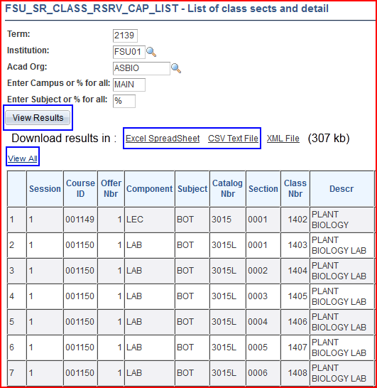
NOTE: If you decide to download the results after you run an HTML query, you can either:
- re-run the query, or
- download the results by clicking the Excel Spreadsheet or CVS Text File options.
Downloading to Excel allows you to sort, format, track, or annotate the data as required. Any changes you identify could then be manually updated in the scheduling system.
FAQs: Downloading Query Results to Excel
Downloading your query results into an Excel spreadsheet is a good way to provide yourself with a quick reference document. However, you may not require all of the data that automatically appears in the spreadsheet upon download. Here are some suggestions to help you refine your take-away document.
How Do I Hide Unnecessary Columns?
Here's an image of a spreadsheet displaying 10 columns-A through J. To hide columns I and J (or any columns of your choosing), do the following:
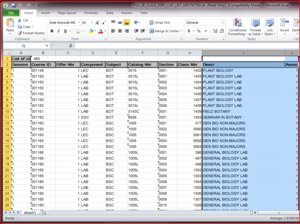
1. Drag the cursor over the letter cells containing I and J. Those columns are now highlighted.
2. Right click the mouse. A pop-up menu appears.
3. Click Hide. Columns I and J become hidden from view.
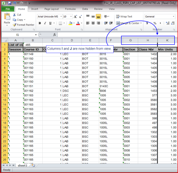
4. To "unhide" them, right click and click Unhide.
How Do I Use Excel's Filter Functionality?
Using the example above, assume you need to filter based on total enrollment (column V).
1. In the menu bar, click the Data tab.
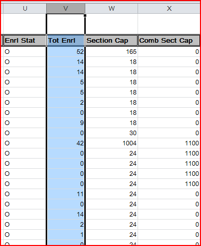
2. Select the range of cells containing the numeric data on which to sort. In this case, click the V letter-cell. The entire column is highlighted.
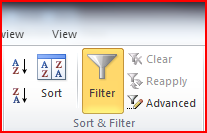
3. In the Sort and Filter group, click Filter. A small down arrow appears in the V letter-cell.

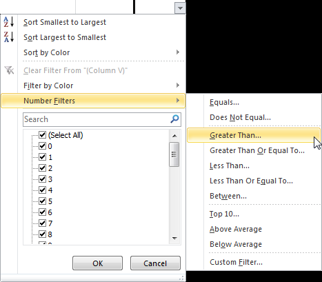
4. Click the down arrow. A menu with filter options appears. In this example, select Number Filters>Greater Than.
5. The Custom AutoFilter dialog box appears. Type 10 in the field adjacent to the is greater than operator.

6. Click OK. The spreadsheet returns, filtered by values greater than 10. However, theses values aren't in order by greater-to-lesser or lesser-to-greater.
7. Click the V letter-cell again. The column is highlighted.
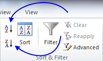
8. In the Sort and Filter group, click either the smallest-to-largest (A>Z) button or the largest-to-smallest (Z>A) button.
9. A warning appears notifying you that if you sort on one column, data in adjacent columns will not travel with the sort action. Ensure that the Expand the selection radio button is selected to have data remain where it should in relation to the new sort.
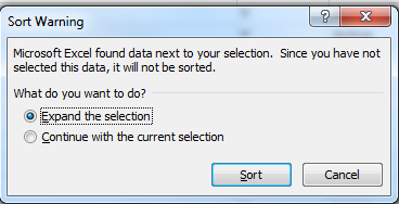
10. Click Sort. The table is now sorted according to total enrollments.
How Do I move the column I just sorted to the A-column position?
In this example, the V column is moved to the A column position.
1. Scroll to the V column and left click in the V letter-cell. The V column is highlighted.
2. Right click and select Cut.
3. Scroll to the A column and left click in the A letter-cell. The A column is highlighted.
4. Right click and select Insert Cut Cells. The new A column appears. Below is an example of a table in which the former V and W rows have been moved to the A and B column positions.
